Statistics is an essential tool when trying to evaluate both the usability and the user experience of a prototype. It allows you to interpret numbers in a systematic way and to communicate your results to the research community.
This chapter will show you a number of statistical methods to analyze the data of your user studies and tell you how to report your results in a scientific publication. We will use a free software called R to do this. This chapter assumes that you know basic programming concepts like variables and arrays.
11.1 Introduction to R
The R software is a free statistics tool with enormous power. It is used around the world by researchers to compute statistics and to visualize their results. R is "command based" which makes it appealing to programmers since you can save snippets of "code" once you figured out a good way of analyzing your experiment so you can robustly repeat the analysis.
11.1.1 Installing R and R Studio
To use R you first have to install it. Find your installation package on the R Homepage, download and install it.
You can run R in a terminal (command shell) or in a dedicated tool called R Studio with a graphical environment. We recommend the latter. Download and install R Studio first: www.rstudio.com
Now start R Studio. You should see something like this:
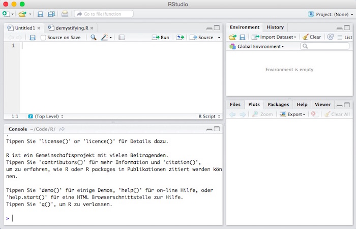
R Studio is still command based (lower left window) but has some more comfort functions. You type your commands in the window with the prompt (the > sign).
Our first command is a simple calculation. Try addition:
> 1 + 2R will output:
[1] 3Next, we will run you through some basic concepts.
11.1.2 Variables
You can introduce variables to store values. You assign a value using the equal sign:
> foo = 3and then output them again
> foo
[1] 3
(If you wonder about the "[1]" - this will be exlained when it gets to vectors.)
Instead of an equal sign = you can also use <- to assign a value to a variable
> boo <- 42
> boo
[1] 42
You can do computations with variables
> foo^2 + 100
[1] 109
You remove a variable with
> rm(foo)11.1.3 Vectors
Since we will work a lot with series of numbers or labels, let's have a look at vectors. A vector is a sequence of e.g. numbers and is defined with the c() function (for concatenate):
> v = c(2, 3, 10)You can look at the vector like this
> v
[1]  2  3 10
A vector can also contain other data like e.g. strings.
> people = c("James", "Harry", "Sally", "Jack")Each vector element has an index number, starting with 1 (not with zero!). The [1] in the output means that this line starts with the element of index 1. You see the point when using a longer vectors:
> w = c(2,2,1,1,3,4,4,4,5,5,6,6,6,5,55,4,4,4)
> w
 [1]  2  2  1  1  3  4  4  4  5  5  6
[12]  6  6  5 55  4  4  4
This shows you that the first index of the upper line is 1 and the first index of the lower line is 12.
A vector of random numbers can be generated with
> rnorm(5)
[1] -0.10859021 -0.06686455 -0.17987425  1.43393312  0.50994595
To open the documentation of an R function you type
> help(rnorm)In R Studio, the help information will appear in the lower right window.
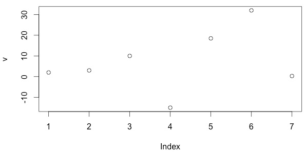
A simple plot of your data can be drawn with
> v = c(-10,0, 5, 7.5, 10)
> plot(v)
Again, the output will appear in the lower right window.
To see examples of an R function you type
> example(plot)We know how to create a vector. You can also do vector arithmetic, i.e. compute with vectors. Usually, operations apply to all elements of a vector.
> a = c(1,2)
> b = c(3,4)

> a + b
[1] 4 6

> a + 2*b
[1]  7 10
Some more vector functions:
> length(a)
[1] 2

> min(a)
[1] 1

> max(a)
[1] 2

> append(a, b)
[1] 1 2 3 4
The following commands generate regular sequences of numbers (as vectors). This is highly useful to quickly generate test data:
> 1:5
[1] 1 2 3 4 5

> 5:1
[1] 5 4 3 2 1

> seq(1, 5, by=.5)
[1] 1.0 1.5 2.0 2.5 3.0 3.5 4.0 4.5 5.0

> rep(5, 3)
[1] 5 5 5

> rep("foo", 5)
[1] "foo" "foo" "foo" "foo" "foo"

> rep(c(1, 2), 5)
[1] 1 2 1 2 1 2 1 2 1 2
11.1.4 Scripts and Files
If you store a sequence of commands in a file, this is called a script and typically has .R as a file extension. To load and execute a script called "myscript.R" you type
> source("myscript.R")Vectors can be accessed in a variety of ways using indeces (starting with 1, not 0!):
> v = c(10, 20, 30, 40)
> v[1]
[1] 10
> v[2]
[1] 20
> v[2:4]
[1] 20 30 40
You can see you current directory (also called working directory) with
> getwd()
[1] "/Users/harryhacker/temp"
And you can go to another directory with
> setwd("../work")You can look at the content of the current directory with
> dir()You write data with
> write.table(v, file="foo.txt")Or with
> write.csv(v, file="foo.csv")And you read tables with
> tab = read.table(file="foo.txt", header=T)11.1.5 Data Frames
A data frame is a table with rows and columns, it can have column names and row names.
You can create a data frame out of vectors. Let's say we have a vector r with ratings and a corresponding vector p with the respective prototype that was rated. We can put this into a table with three columns named "prototype", "rating" and "time".
> p = c("a", "a", "b", "b")
> r = c(4, 3, 3, 5)
> t = c(.5, .3, .7, .2)
> df = data.frame(prototype = p, rating = r, time = t)
> df
        prototype rating time
1         a      4  0.5
2         a      3  0.3
3         b      3  0.7
4         b      5  0.2
You can access columns with the following notation:
> df$prototype
[1] a a b b
Levels: a b

> df$rating
[1] 4 3 3 5

> df$time
[1] 0.5 0.3 0.7 0.2
You can retrieve the column names with
> names(df)
[1] "prototype" "rating"    "time"
To read a data frame from a file there are two functions. If the data is delimited by comma (CSV file) use
> df = read.csv(FILENAME, header = T)If the data is delimited by tabs use
> df = read.delim(FILENAME, header = T)In both cases I assumed that the column names are listed on the first line (header).
You can access a single cell like with a matrix. Always remember that in R indeces for data structures start with 1 and not with 0.
> df[1,1]
[1] a
Levels: a b
If you leave the first index empty, it means "all row elements", so that you get the first column:
> df[,1]
[1] a a b b
Levels: a b
Likewise with the second index: you get the whole row:
> df[1,]
      prototype rating time
    1         a      4  0.5
This is called slicing. You can also retrieve the first two rows like this:
> df[1:2,]
  prototype rating time
1         a      4  0.5
2         a      3  0.3
For retrieving columns you can also use the column names:
> df[, c("rating", "time")]
  rating time
1      4  0.5
2      3  0.3
3      3  0.7
4      5  0.2
11.2 Descriptive Statistics
The purpose of descriptive statistics is to summarize a (possibly large) set of numbers by a single number because - obviously - it is hard to look at a huge set of numbers (e.g. 100 user ratings for a product on a scale of 1 to 5) and figure out what it all means.
Examples for descriptive statistics are: min, max, mean or variance.
11.2.1 Measures of central tendency
Measurements often cluster around certain intermediate values. Given a set of values:
- the mean is the average of all values
- the median is the one value of this set which is bigger than half of all values and smaller than half of the values
- the mode is also one value of the set - it is the most frequently occurring one
In R, the mean of a range of numbers can be computed with
> v = c(2, 3, 10)
> mean(v)
[1] 5
The median is also available and can be quite different from the mean:
> v = c(1, 1, 1000, 3, 4)
> median(v)
[1] 3
> mean(v)
[1] 201.8
11.2.2 Measures of variability
Apart from the central tendency you might be interested in the question of how spread out the data are. For instance, if 100 users give ratings for product X on a scale of 1 to 5, it makes a difference if
- all users say 3
- half of the users say 1, the other half say 5
In the first case, you are pretty sure the product is average. In the second case, the users seem to be undecided. Note, though, that in both cases the mean is 3!
> a = c(1, 1, 1, 5, 5, 5)
> b = c(3, 3, 3, 3, 3, 3)
> mean(a)
[1] 3
> mean(b)
[1] 3
Therefore, we need a characterization of data width, variability or spread. The higher the spread, the less dependable the data is for the understanding of the general population.
A first idea would be to look at the minimum and maximum of the data sets. This is also called the range. In R:
> range(a)
[1] 1 5
> range(b)
[1] 3 3
The range is not very robust because the minimum and maximum values could be quite exceptional:
> c = c(3, 3, 3, 3, 1, 5)
> range(c)
[1] 1 5
A more robust (and a single) value is the variance. The variance looks at the difference between each value and the mean value. To be precise, it is the squared difference between each value and the mean, divided by the number of values minus one. In R:
> var(a)
[1] 4.8
> var(b)
[1] 0
As you can see, the variance tells you that value set b has much lower variance/spread than set a. The standard deviation is the square root of the variance and is actually more commonly used. In R:
> sd(a)
[1] 2.19089
> sd(b)
[1] 0
In a scientific paper you report mean (M) and standard deviation (SD) like this (in case we have the data in a):
"We asked 6 students to rate our prototype on a scale of 1..5 and the results were quite mixed (M = 3, SD = 2.19)"
11.3 Testing for Significance: t-test
Apart from simply summarizing your data, statistics can be used to interpret your data. For our purposes, this usually means comparing two average values, e.g. the average rating for prototype A versus the average rating of prototype B.
11.3.1 Comparing means
Imagine we do a user study to compare two prototypes A and B. We simply ask users to tell us how they like a prototype on a scale of 1 (not at all) to 5 (very much).
There are two ways to do design our experiment:
- We ask 6 users to rate A and 6 other users to rate B (between-subjects design)
- We ask 10 users to rate both A and B (within-subjects design)
Let's assume the first case, i.e. we have a between-subjects design. We store the answers of the first 6 users in a and the ones of the other 6 in b:
> a = c(3,3,3,3,3,3,4)
> b = c(4,4,4,4,4,4,3)
The answers look quite consistent, with only one exception each. Let's look at the mean values:
> mean(a)
[1] 3.142857
> mean(b)
[1] 3.857143
In table form:
| A | B | |
|---|---|---|
| mean | 3.14 | 3.86 |
The difference is not big but I would trust that prototype B is more popular from the reply pattern.
Let's look at another experiment with prototypes C and D. The answers look different this time:
> c = c(1,5,3,3,3,3,4)
> d = c(1,5,5,5,4,4,3)
This time I am not sure I can trust the data. Let's look at the means:
> mean(c)
[1] 3.142857
> mean(d)
[1] 3.857143
In table form:
| A | B | C | D | |
|---|---|---|---|---|
| mean | 3.14 | 3.86 | 3.14 | 3.86 |
The means are the same as in the case of A/B. However, my mistrust stems from the high variation in the data. So let's look at the standard deviation of a and c:
> sd(a)
[1] 0.3779645
> sd(c)
[1] 1.214986
So, yes, it is different. What about b and d?
> sd(b)
[1] 0.3779645
> sd(d)
[1] 1.46385
Again, quite different. Let's have a look at all the numbers:
| A | B | C | D | |
|---|---|---|---|---|
| mean | 3.14 | 3.86 | 3.14 | 3.86 |
| sd | 0.38 | 0.38 | 1.21 | 1.46 |
We can see that our intuition is reflected in the standard deviation. Is there a way to find out whether the difference between a/b or c/d is significant? The answer is yes. We utilize the t-test.
11.3.2 t-test and significance
The t-test compares two mean values and tells us whether these values are different to a significant degree, considering the variance in the data. In other words: if we would acquire more and more data would the difference remain or maybe go away?
In R, you compute the t-test like this:
> t.test(a,b)

    Welch Two Sample t-test

data:  a and b
t = -3.5355, df = 12, p-value = 0.004104
[...]
R shows us more but the interesting bit is the p-value (or simply p). This is the probability that the null hypothesis (H0) is true. The null hypothesis is that the two distributions actually have an equal mean value (and we just don't have enough data to see it). Since the p-value is low we can conclude that the the means of a and b are significantly different (i.e. if we had more data the values would likely still be different). Significance has been defined by the research community as p being smaller than 0.05.
If we do the same for our other two prototypes C/D, we get:
> t.test(c,d)

    Welch Two Sample t-test

data:  c and d
t = -0.9934, df = 11.606, p-value = 0.3408
Let's remember again what we found out about the data in terms of descriptive statistics. The variation of the C/D data is much higher than the variation of A/B.
| A | B | C | D | |
|---|---|---|---|---|
| mean | 3.14 | 3.86 | 3.14 | 3.86 |
| sd | 0.38 | 0.38 | 1.21 | 1.46 |
And here are the results from our two t-tests:
| A vs B | C vs D | |
|---|---|---|
| p-value | 0.004 | 0.34 |
You can see that p is much higher for C/D (and clearly larger than 0.05) so there is a chance that the two means are actually equal (= null hypothesis) and simply because our data sets are so small they appear to be different.
Reporting Results
In a scientific paper you report a t-test like the one for A/B like this (the value in brackets after the t are the degrees of freedom or df):
"Our subjects liked prototype B slightly better as revealed by a t-test, t(12) = -3.54, p < .05."
As you can see, you only report p < .05 or p < .01. This is called the level of significance.
11.3.3 Levels of significance
It is important to note that the significance level of 0.05 has been arbitrarily set by humans. However, in research people stick very strictly to this number. If you have a very low p value (which is normally what you want) smaller than 0.01 you can speak of a highly significant result.
These boundary values (0.05 and 0.01) are also called alpha level. So we can say that for a significant result we apply an alpha level of 0.05 and for a highly significant result we require an alpha level of 0.01.
11.3.4 Paired samples t-test
Let's go back to the two possible designs of our study:
- We ask 6 users to rate A and 6 other users to rate B (between-subjects design)
- We ask 10 users to rate both A and B (within-subjects design)
In the above example we had two prototypes A and B and each prototype was rated by a different group of people (between-subjects design). This experimental design actually requires that the two groups are comparable and to ensure this one needs a high number of subjects.
If the same person compares both prototypes (within-subjects design), this leads to a clear results with much fewer subjects. Now the numbers have a slightly different meaning:
> a = c(3,3,3,3,3,4)
> b = c(4,4,4,4,4,3)
This time the first number of each data set refers to the rating of the same person no. 1. The second numbers of each were obtained from the same person no. 2 and so on. On could also say that these numbers are paired. This makes a difference both in terms of interpretation and in terms of computation. We need to use a different test called the Student's t-test for paired samples:
> t.test(a, b, paired=T)

    Paired t-test

data:  a and b
t = -2, df = 5, p-value = 0.1019
We see that the p-value is higher than in our previous t-test (p = 0.004104). In fact, the difference in ratings is not even significant!
Well, when you look at the data you may find it striking that the last participant rated exactly the other way round compared to everyone else - so she clearly favored prototype B. What if the data looked like this:
> a = c(3,3,3,3,3,4)
> b = c(4,4,4,4,3,4)
Now we don't have this "inverse" person but we have two "indifferent" people instead. This directly impacts the result of the t-test:
> t.test(a, b, paired=T)

    Paired t-test

data:  a and b
t = -3.1623, df = 5, p-value = 0.02503
This time, our result is significant (p < 0.05). So with paired data the order of the numbers obviously matters a lot.
Example with a CSV file
If we have questionnaire results as a file called "data.txt":
    Q1,Q2,Q3,Q4
    5,3,3,1
    2,1,2,4
    3,5,4,2
    4,4,5,2
    5,5,2,3
    4,5,5,1
We can read the data thus:
> d = read.csv("data.txt", header=T)Now to compute the difference between Q1 and Q4 we compute a paired t-test:
> t.test(d$Q1, d$Q4, paired=T)And get this:
    Paired t-test

    data:  d$Q1 and d$Q4
    t = 1.9764, df = 5, p-value = 0.1051
    alternative hypothesis: true difference in means is not equal to 0
    95 percent confidence interval:
    -0.5010383  3.8343716
    sample estimates:
    mean of the differences
    1.666667
Reporting Results
In a scientific paper you mention the variant of the t-test (here: paired samples):
> "Our subjects liked prototype B slightly better as we could show with a _paired samples_ t-test, t(5) = -3.16, p < .05."11.4 Testing for Significance: ANOVA
A t-test only works if you have two prototypes. What if there are more?
11.4.1 More than two samples: One-way ANOVA
Let's say we now compare three prototypes instead of just two: A, B and C. We collect ratings for each prototype. We may think: well, just compute three t-tests for A-B, B-C and A-C! The problem with this is that we introduce the possibility that we get a significant result by chance, simply because to compute so many t-tests. So this approach is not allowed.
Therefore, we use the so-called Analysis of Variance, short ANOVA, to find out whether the three means differ. This technique will tell us only if there is a difference somewhere between the three means. It does not tell us where this difference lies (between A and B, between B and C, between A and C). For the latter we have to run post hoc tests after the ANOVA analysis.
Some terminology: for the fact that we look at different prototypes, we call "prototype" a factor with three levels (A, B and C). This is why here we are dealing with a One-way ANOVA. We are only looking at a single factor. We we wanted to examine gender effects and thus partition our subjects in male/female for analysis, we would then have two factors (prototype and gender). This calls for a different type of ANOVA called Factorial ANOVA.
For easy use in R, store the rating in the following way as a file called e.g. "ratings.csv". Every rating appears on one line. We have two attributes: prototype (A, B, C) and rating (1..5).
prototype,rating
A,1
A,2
A,2
A,1
A,2
A,1
A,1
A,2
A,2
A,1
B,5
B,3
B,2
B,4
B,2
B,1
B,2
B,3
B,5
B,2
C,1
C,2
C,2
C,3
C,1
C,5
C,3
C,3
C,1
C,1
Read the data into R:
anova.data = read.csv(file)The following command makes the two attributes prototype and rating accessible as variables in R:
attach(anova.data)Now we can look at the data in table form. E.g. how many ratings we have for each prototype:
table(prototype)
prototype
  A  B  C
10 10 10
We can also compute the mean for each prototype:
tapply(rating,prototype,mean)
  A   B   C
1.5 2.9 2.2
Or the standard deviation:
tapply(rating,prototype,sd)
        A         B         C
0.5270463 1.3703203 1.3165612
We can plot it as a whisker plot which displays the median:
plot(prototype,rating)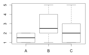
Finally, we run the ANOVA:
anova.aov = aov(rating ~ prototype, data = anova.data)
summary(anova.aov)
            Df Sum Sq Mean Sq F value Pr(>F)
prototype    2    10.8   4.900    3.78 0.0357 *
Residuals   27   35.0   1.296
---
Signif. codes:  0 ‘***’ 0.001 ‘**’ 0.01 ‘*’ 0.05 ‘.’ 0.1 ‘ ’ 1
We can see under Pr that there is a significant interaction (p < 0.05) between A, B and C. However, we don't know whether it stems from A and B or from B and C or from A and C.
Post Hoc Tests
So now we run post hoc tests to find out which prototypes are different to which degree. We basically come back to our first idea to compute something like a t-test for every combination of two prototypes (A-B, A-C, B-C). When we do this we have to respect the fact that a significant result is more likely to come up by chance. Therefore, we need to be stricter when judging "significance". We can do this in two ways. We either lower our Alpha level (0.03 instead of 0.05) or we could increase our p-values. The latter is called Bonferroni adjustment and needs to be specified in the command:
pairwise.t.test(rating,prototype,p.adj="bonferroni")
    Pairwise comparisons using t tests with pooled SD

data:  rating and prototype

  A     B
B 0.032 -
C 0.542 0.542

P value adjustment method: holm
In table form:
| A | B | |
|---|---|---|
| B | 0.032 | |
| C | 0.542 | 0.542 |
In the table we can see the p-values of the three possible pairwise combinations. We can see that only A and B differ significantly.
Apart from Bonferroni adjument there are further adjustment methods that can be used in R (for p.adj): holm, bonferroni, hochberg, hommel, BH, BY. The latter two stand for "Benjamini-Hochberg" and "Benjamini-Yekutieli". An adjustment method is either more conservative (i.e. it is harder to get significant results) or more liberal (i.e. it is easier).
Take a look again at the means:
tapply(rating,prototype,mean)
A   B   C
1.5 2.9 2.2
So now we can say that in our data, prototype B is rated significantly higher (mean rating of 2.9) than prototype A (mean rating of 1.5). In contrast, the difference between prototype C (mean rating 2.2) and B could be a mere coincidence.
Reporting Results
In a scientific paper you an ANOVA you report the F-value with two degrees of freedom (Df) and the p-value. From the pairwise comparisons (post hoc tests) you report the adjustment method (e.g. Bonferroni or Holm) and the significant pairs.
"An ANOVA showed that ratings differ significantly for the three prototypes, F(2, 27) = 3.78, p < .05. Post-hoc tests - corrected with the Holm method - revealed that prototype A was clearly preferred over B (p < 0.05)."
11.4.2 Two-way ANOVA
To make it even more complicated, what if you have two prototypes and want to find out if there is a gender effect, i.e. if women prefer prototype A whereas men prefer prototype B. In this case, we have two factors: gender and prototype. When we have more than one factor we say that the experiment has a factorial design and the analysis method is a two-way ANOVA.
For each factor we have levels:
- factor gender has two levels: female (F) and male (M)
- factor prototype also has two levels: A and B
We start with the case that there are four groups: female/A, female/B, male/A, male/B. This is called an independent factorial design.
Possible Outcomes: Main Effects and Interactions
We can first think about what we could possibly find out. Our only dependent variable is rating. This is the measurement that we take in our experiments. Our two factors are gender and prototype.
First, we could find out that gender has an impact on ratings, e.g. "women always rate higher than men". This would be called a main effect. It has nothing to do with prototypes.
Second, we could find out that prototype has an impact on ratings. This is the same as the example for the one-way ANOVA. E.g., "prototype A is always better rated than prototype B". This would also be called a main effect.
So in general, a main effect is an effect that is restricted to one factor.
Third, we could find out that gender and prototype interact, e.g. "women rate prototype A higher, whereas men rate prototype B higher". This is called an interaction.
Data
The data could look like this:
gender,prototype,rating
F,A,4
F,A,5
F,A,3
F,A,5
F,A,5
M,A,1
M,A,1
M,A,2
M,A,2
M,A,1
F,B,5
F,B,3
F,B,2
F,B,4
F,B,2
M,B,1
M,B,2
M,B,3
M,B,3
M,B,2
Prerequisites
First, we have to check whether the four groups are not too heterogeneous by analyzing and comparing their respective variances. This is done with a Levene Test. To use this you have to install the package "car":
install.packages("car")After installation, tell R to use it
library(car)Call the test with
leveneTest(rating, interaction(gender,prototype), center = median)You will see
Levene's Test for Homogeneity of Variance (center = median)
      Df F value Pr(>F)
group  3  0.6667 0.5847
      16
What we want here is a non-significant result. Since the p-value is clearly above 0.05 the test shows that we can apply an ANOVA here.
ANOVA
Compute the model:
anova.model = aov(rating ~ prototype*gender, data = anova.data)Run a Type III test:
Anova(anova.model, type="III")

Response: rating
                 Sum Sq Df  F value    Pr(>F)
(Intercept)        96.8  1 110.6286 1.354e-08 ***
prototype           3.6  1   4.1143 0.0595074 .
gender             22.5  1  25.7143 0.0001135 ***
prototype:gender    5.0  1   5.7143 0.0294735 *
Residuals          14.0 16
---
Signif. codes:  0 ‘***’ 0.001 ‘**’ 0.01 ‘*’ 0.05 ‘.’ 0.1 ‘ ’ 1
There is a highly significant main effect of gender (p < .01). There is no main effect on prototype.
However, there is an interaction between gender and prototype (p < .05).
11.5 Testing for Correlation
Let's assume you have numerical data of two different types that you have measured in experiments, e.g.
- amount of training vs. error rate
- number of choices in a menu vs. time it takes to reach a decision
- amount of time spent with a system vs. liking for the system
For each example case above you would like to know whether there is a systematic relationship between the numbers. You hypothesis could be something like:
- "The higher the amount of training, the lower the error rate"
Not only do you want to prove this hypothesis, you would also like to derive a model from your data which predicts - for future interactions - the error rate given a certain amount of training.
11.5.1 Regression
Let's look at a really simple toy example for the case of training time vs. error rate (these are not real measurements):
    > time = c(1, 2, 5, 3, 2, 2.5)
    > errors = c(12.5, 5.3, 1.5, 3.3, 6.1, 4.6)
The values reflect the amount of time spent with the system (in hours) and the error rate (in %). Of course, the length of the two vectors must be equal. First of all, we can plot the data:
> plot(time,errors)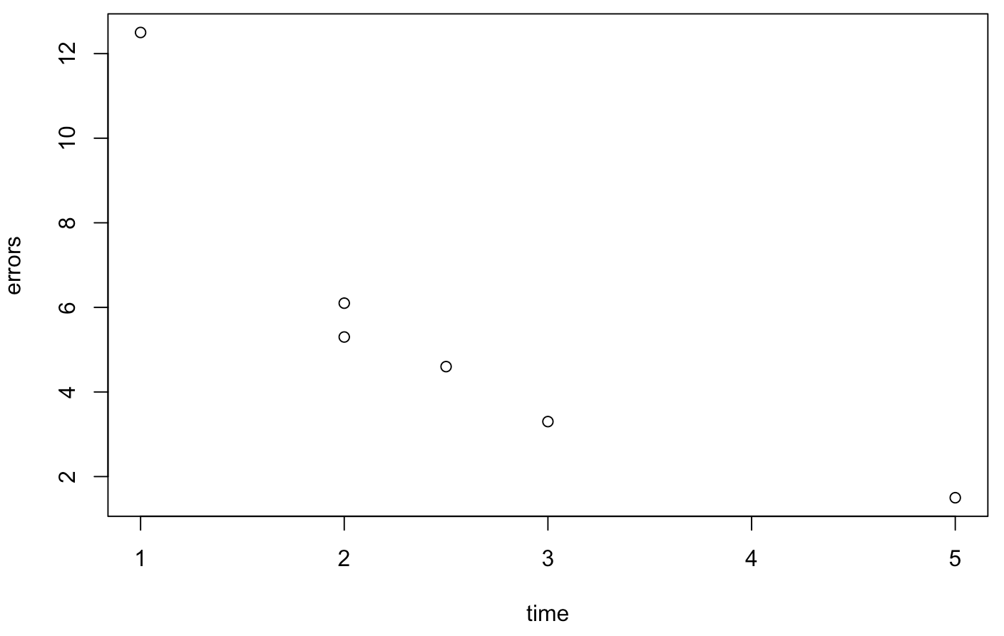
We see that there is probably a linear relationship between the data. We can let R try to compute a linear model. The method for obtaining this model is called regression. Note the order of the two data: the outcome variable (errors) comes first, the predictor variable (time) comes second:
> model = lm(errors ~ time)Now we can look at the result with
> summary(model)The interesting items are the intercept of 11.673 and slope of -2.37 (this appears as "time" here). These are the components of a linear formula that you may remember from school:
y = a * x + bwhere a is the slope and b is the intercept (where the line hits the y axis). In our case the line is defined by:
errors = -2.37 * time + 11.673This corresponds to what is called a trendline. You can add the trendline to your plot with
> abline(model)11.5.2 Correlation Coefficient
The other important figure from summary(model) is the correlation coefficient which tells you how good your predictions with this model will be (graphically speaking: how close to the trendline all the dots are). This is the so-called R-squared value. R is the so-called Pearson correlation coefficient. So we have to take the square root to obtain it:
    > sqrt(0.7282)
    [1] 0.8533464
If R is close to 1, the relationship is almost perfectly linear. If it is close to 0, there is practically no linear relationship. In our example we obain an R value of 0.85 which confirms our hypothesis that there is a linear relationship between training time and error rate.
To round this of we also have an analysis of variance (ANOVA) that is run:
F-statistic: 10.72 on 1 and 4 DF, p-value: 0.03068Since the p-value is smaller than 0.05 we can call this a significant result.
11.6 Further Reading
11.6.1 Statistics
I can highly recommend the following book for anyone who wants to understand statistics with a focus on testing:
- T.C. Urdan (2010) Statistics in Plain English, 3rd edition, Taylor & Francis, 224 pages.
For people who prefer video there is a brilliant playlist by Professor Leonard:
11.6.2 R
For statistics in R there is this very comprehensive volume:
- A. Field, J. Miles (2012) Discovering Statistics Using R, Sage Publications, 992 pages.
There are plenty of resources for R online:
- Introduction to R (PDF) by W. N. Venables, D. M. Smith and the R Core Team
- A (very) short introduction to R (PDF) by P. Torfs and C. Brauer